Singlearity: Using A Neural Network to Predict the Outcome of Plate Appearances

Image credit: Jim Rassol-USA TODAY Sports

We trained a neural network on the last nine years of Major League Baseball games. It learned to weigh large amounts of data to predict the outcomes of plate appearances more accurately than previous techniques. The neural network also learned the strategies and rules of the game, and used this understanding to enhance prediction quality. We believe our approach can be used to make more effective pre-game and in-game strategy decisions, and to provide for more accurate game simulations.

Our model, Singlearity-PA (pronounced single-air-ity), improves upon previous techniques, such as log5, in that it:

• Provides substantially more accurate predictions, performing better than log5 across every type of prediction and across matchups that involve both veteran players and new players.
• Incorporates the widest range of predictive data, including platoon statistics, pitch count, ballpark characteristics, and batted ball exit velocity, among others.
• Uses game state data, (e.g. bases loaded with one out in the 8th inning) aiding in both prediction accuracy and specificity (e.g. sacrifice fly).
• Presents an easy framework to continuously improve the model by incorporating new types of data.

You can access a live version of Singlearity-PA to predict your own batter vs. pitcher matchups at www.singlearity.com.

Introduction 

Imagine yourself as a team manager facing these difficult decisions:

• Tie game, bottom of the ninth, one out and bases loaded. Your right-handed closer is on the mound, facing a left-handed batter whom he has completely dominated in the past. However, you have a left-handed pitcher in the bullpen who often induces double plays. Should you switch the pitcher?
• You are in the middle of a long road trip facing an upcoming 4-game series against your league rival, but your catcher is in need of a rest. You know the projected opposing starting pitchers for the series. Which is the best day for your catcher to take a rest?

These are just two examples of questions that any team might face during the course of a season.

Evaluating a batter vs. pitcher matchup is one of the core problems driving baseball strategy. Knowing the odds that the plate appearance (PA) will result in a double-play vs. a strikeout vs. a home run can affect many aspects of the game, such as optimization of the batting order, selection of a relief pitcher, or the decision to intentionally walk a batter, to name just a few. Additionally, techniques such as Monte Carlo game simulation rely on the presumption of accurate batter vs. pitcher simulations.

With the advent of large scale data sets, as well as more efficient ways to ingest, analyze, and model the outcomes, we now have the ability to go far beyond generalized strategies, and to make custom predictions based on the players and situations. The era of accurate, specific predictions is upon us!

Previous Techniques 

Predicting head-to-head outcomes is a common theme in many sports. log5 has been a widely used technique for predicting head-to-head outcomes in baseball. It was originally devised by Bill James as a way to predict the outcome of a game based on two teams’ respective win-loss percentages. James later extended the log5 method to predict the probability of an outcome (hit vs. no-hit) for a particular batter vs. pitcher matchup. log5 uses historical statistics for batter, pitcher and league average to predict the outcome of plate appearances.

Matt Haechrel later created a generalized equation for log5 to extend the possible plate appearance outcomes to more than hit vs. no-hit predictions, so that it could predict the probability of seven types of PA outcomes for each batter vs. pitcher matchup^[1]: out, single, double, triple, home run, walk and hit-by-pitch. Haechrel’s equation relied upon 365-day average rate-per-plate-appearance of each of the seven events for the batter, pitcher, and league. Haechrel’s equation is:

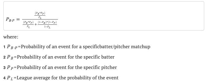
While the notation for this equation is somewhat intimidating, Haechrel’s log5 formula computes batter vs. pitcher matchups in a straightforward manner. However, with that simplicity comes some tradeoffs in accuracy and applicability. Some of the natural limitations of this formula include:

• A large amount of batter and pitcher historical data is required to produce accurate results.
  • In his paper, Haechrel predicts a plate appearance’s outcome only when the batter and pitcher have at least 502 plate appearances or batters faced, respectively, during the previous season. From 2011-2020, only 18.7% of plate appearances fell into this category. To examine what happens if we apply the formula to players with fewer PAs, consider the extreme example of a new player who has been up to bat 20 times, but has not yet hit a home run. log5 will predict this player has 0% chance of hitting a home run. Similarly, log5 will predict a player who has one PA and one HR to have a 100% chance of hitting a HR.

• Data that has been shown to be important in affecting outcome probabilities is ignored, for example:
  • Left-handed vs. right-handed matchups that drive much of the strategies around lineups and substitutions.^[2]
  • Ballpark characteristics – for example, games at the Phillies home field, Citizens Bank Park, produce 84% higher home run rates than games at the Giants’ home field of Oracle Park regardless of which teams are playing.^[3]
  • Players’ speed and position are correlated with probabilities at the plate.
  • Weather factors, such as temperature, humidity and wind direction affect the probability of different outcomes.^[4]
  • Additional, more modern statistics that are becoming widely available, such as batted-ball exit velocity, can potentially be used as well.

• Predictions do not account for the game state. For instance, based on data from 2011-2019, in a tied game with two outs and the bases loaded in the bottom of the ninth, a batter has only a 3.4% chance of a walk. In contrast, in a tied game in the bottom of the ninth with one out and runners on 2nd and 3rd, the batter has a 45.7% chance of a walk, intentional or not.

• All possible PA outcomes are combined into only seven possible outcomes, thus eliminating the possibility to differentiate different types of PA outcomes, such as double play, sacrifice fly, or a sacrifice bunt.

Introduction To Neural Networks 

To deal with the complexity of making sense of our data for predictions, we turn to artificial neural networks.

To understand where neural networks fit in among the hierarchy of artificial intelligence, we describe:

• Machine learning as a branch of Artificial Intelligence that allows “computers the ability to learn without being explicitly programmed.”^[5] This is in contrast with expert systems, in which a group of domain experts attempt to understand input data and reason about how to map the input into the expected results.
• Supervised learning is a subset of machine learning in which we are given an input data set along with a set of “correct” answers, and the computer attempts to learn the rules so that it can make predictions about future data.
• Artificial neural networks as a type of supervised learning implemented by building an internal representation that tries to mimic the computation done in the human brain. Neural networks have been successfully used in a variety of applications including image recognition, automated game playing, and natural language processing. The goal of a neural network is to predict output values based on input values.

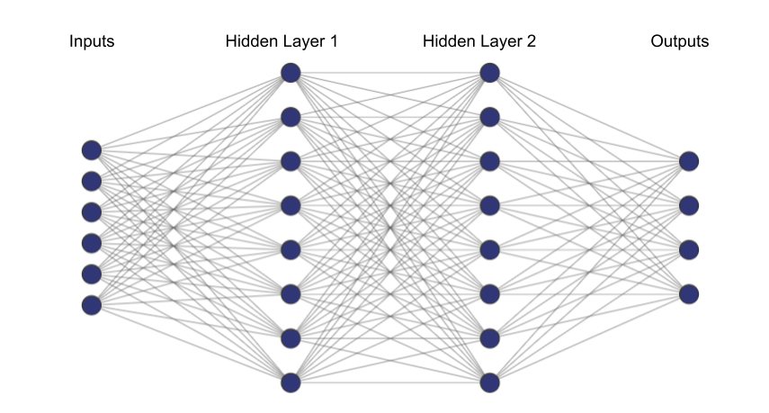
The image above shows an example of a simple neural network whose architecture consists of 6 inputs, 2 hidden layers of 8 nodes each, and 4 outputs. Once the architecture of a neural network has been chosen, it can be trained using supervised learning. In supervised learning, random weights are initially assigned to each edge of the network. These weights, along with the inputs, determine the output values. The network is trained by feeding it input values and the “correct” output values, and the network adjusts the weights of the edges so it can correctly predict outputs. For instance, in the network above, the six inputs could be the batter and pitcher’s batting average, slugging average, and on-base percentage, respectively, and the four outputs could be the probability that the result of the plate appearance is a home run, strikeout, walk, or “other” event, respectively.

Neural networks have at least two properties that make them more successful than other types of prediction models:

• Neural networks, such as Singlearity-PA, excel despite having little domain knowledge. For example, baseball experts build models that try to weigh the importance of different types of statistics, such as recent vs. old vs. head-to-head vs. league average vs. platoon. The goal of a neural network is to discover these subtle relationships without requiring any specific understanding of the baseball domain.
• Neural networks are able to easily incorporate new types of data and determine their usefulness. Scaling to incorporate new data will become a critical feature of any prediction system because the amount of MLB data available for analysis is increasing dramatically. For example, when MLB began reporting advanced statistics with Statcast in 2014, the amount of baseball data in 2014 alone exceeded all the previous data in the prior history of the sport.^[6] Baseball is part of the Information Explosion^[7] and new tools must be created and adapted to exploit this flood of data.

Training Singlearity-PA

To train our neural network, we used pitch-by-pitch Statcast data from 2011-2019.^[8] This consisted of 1.66 million plate appearances played during 21,865 regular season games over 1,627 different calendar days. Using best practices, we split the 1,627 calendar days so that the plate appearances of 60% of the dates were used for training data, 20% for validation data, and 20% for test data. The neural network was trained using the training data and the architecture of the neural network was adjusted by looking at how well the network generalized to correctly predicting results on the validation data. With our finalized architecture, we measured the predictive power of the neural network against the test data.

After experimentation, we chose a neural network architecture that consisted of three types of layers: 

• Input Layer: 79 inputs representing the data that we deemed important for predicting PA outcomes
• Hidden Layers: Two hidden layers of 80 nodes each that the network used for its internal learning process
• Output Layer: 21 outputs representing the possible unique PA outcomes as defined in statcast

The neural network’s task was to use the 79 inputs to predict values for each of the 21 outputs, where each output represented the probability of that PA outcome.

The 79 input fields for each plate appearance were divided as follows:

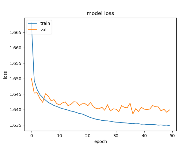
We used categorical cross entropy as the loss function of our network. As we trained our network, we needed to make sure that the model did not overfit the data. Overfitting during training is characterized by a model loss error rate which decreases on the training data, but which rapidly diverges from the error rate when applied to the validation data. Overfitting is problematic because it means that the model will not be able to generalize the predictions to handle new data. Because we had a large sample of data to train the network and a relatively simple neural network architecture, we did not expect the network to overfit the data. As shown in the graph below, we can see that the loss for both the training and validation data remain comparable to each other, which indicates that the neural network did not overfit the training data.

Did Singlearity-PA “Learn” Baseball?

To get a sense of Singlearity-PA’s predictions, see the figure below which shows Charlie Blackmon batting against Max Scherzer in the following game situation:

Location: Coors Field

Inning: Bottom of 5th

Score: Tied

PItch Count: 70

Outs: 1

Baserunners: Runner on 1st

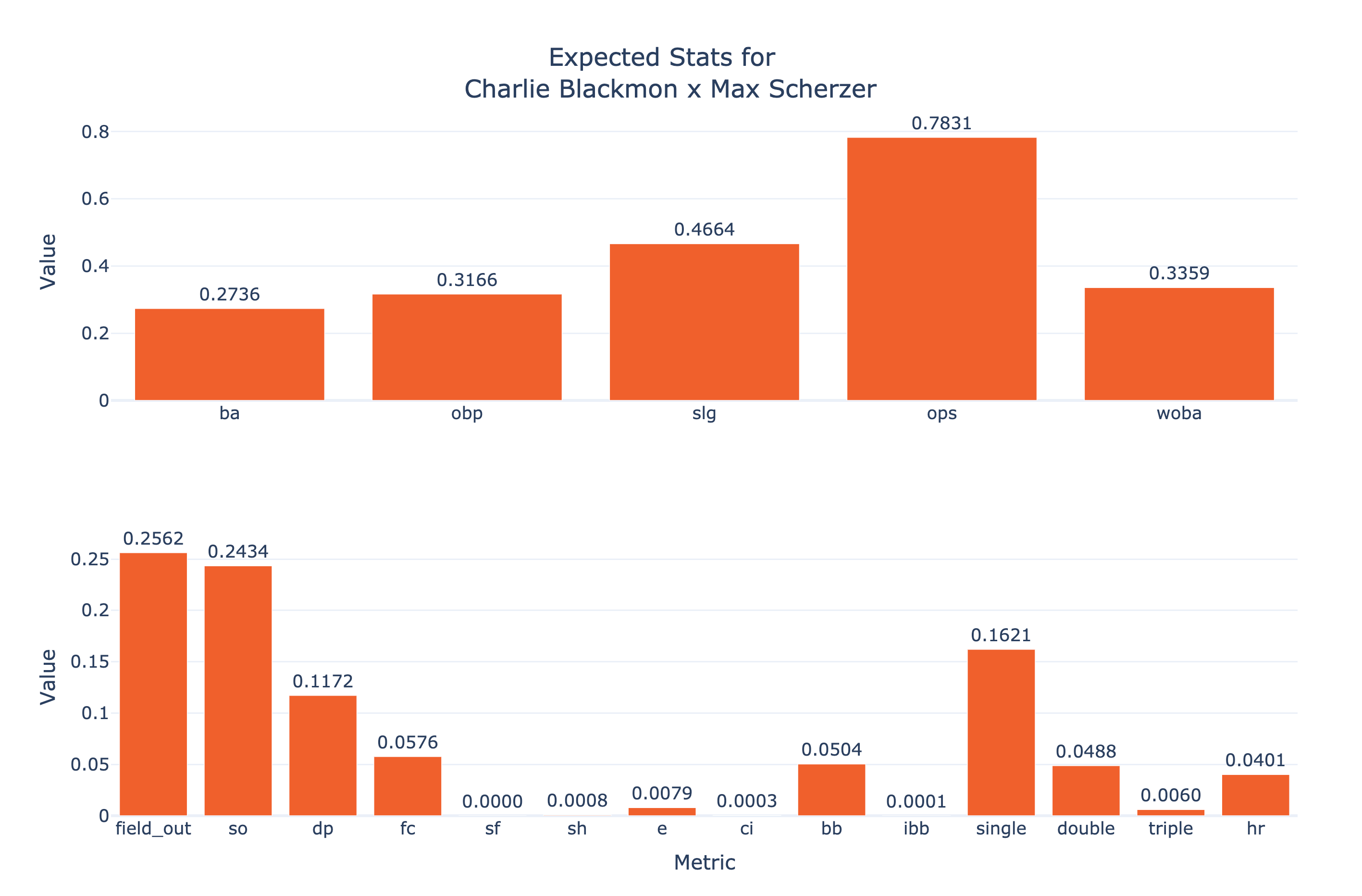
Now, to understand just how much these predictions can vary depending on the game state, let’s vary the baserunners and outs and observe the changes in the figure below. The baserunners/outs are shown in the top left corner. Notice, for instance, how much variation there is in Blackmon’s batting average (“ba” on the diagram below) depending on the state of baserunners and outs. Also, notice that the probabilities for events such as double play (“dp”), sacrifice fly (“sf”) and fielder’s choice (“fc”) seem, at least visually, to correspond to realistic outcomes in a game.

Before we examine the results in a more quantitative way, let’s do a couple of quick sanity checks to test Singlearity-PA’s understanding of the game, by:

• Observing that Singlearity-PA will not predict a double play when there is no one on base. Indeed, of the 946K PAs that occurred with no one on base since 2011, Singlearity-PA’s maximum predicted probability of a double play during these PAs was 1 x 10^-8.
• Observing that Singlearity-PA understands when a sacrifice bunt is likely to occur. Most casual baseball fans know that there is a high likelihood of a sacrifice bunt when a pitcher is at bat with a runner on first base only and less than two outs. In fact, of 6308 occurrences since 2011, the plate appearance resulted in a sacrifice bunt 49.6% of the time^[13]. For these same “high sacrifice probability” situations, Singlearity-PA predicts a sacrifice bunt with an average expected value of 59.7%.

Quantitative results 

Singlearity-PA’s quantitative comparison to log5 are shown in the tables below. To get an intuitive sense of both models’ error rates, we compared them to an extremely simplistic model for league averages, in which we assumed the probabilities for plate appearance outcomes correspond to the league’s average expected outcomes for the year.

Because it was claimed that log5 techniques would work best for plate appearances in which there were substantial historical stats for both the batter and pitcher, we examined how both Singlearity-PA and log5 worked when used to predict PAs with varied amounts of historical data available. We categorized each PA into one of the following categories:

• Extensive predictive data: Both batter and pitcher had >=502 PA or opposing PAs, respectively in the last 365 days.^[14]
• Little predictive data: Either the batter or the pitcher had <100 PAs in the last 365 days.
• Some predictive data: All other PAs.

It is important to note that from 2011-2019 only 18.7% of PAs fall into the “Extensive predictive data”, while 60.1% of PAs fall into “Some predictive data” and 21.2% fall into “Little predictive data”. Thus, it is critical that any technique be able to produce accurate results for PAs beyond just the “Extensive predictive data” category.

We’ve chosen to show the error rates for a few of the different types of predictions below, although it should be noted that the measurements of all types of predictions produced similar results. First, let’s look at the ability to predict specific PA outcomes.

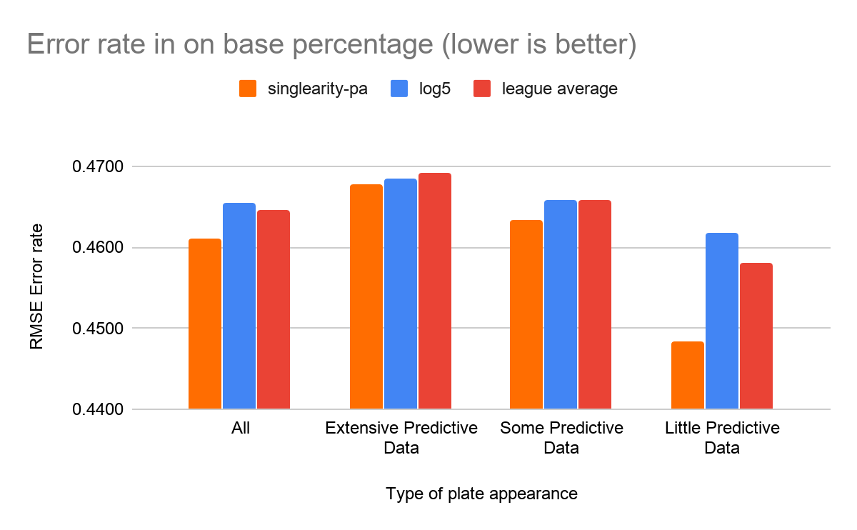
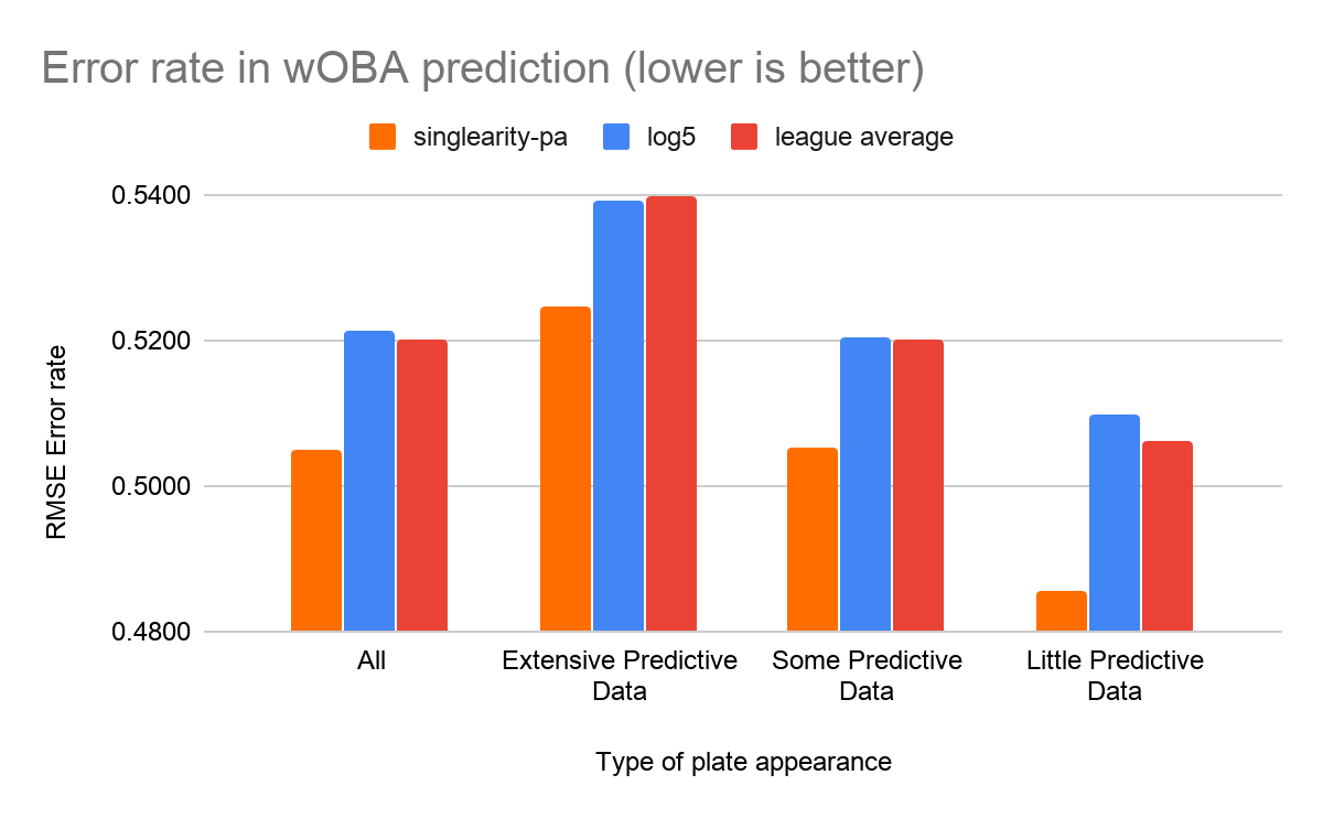
Second, we compare the ability to predict composite stats. For instance, to predict the expected on-base percentage of a PA, we add up the probabilities of all events that correspond to an on-base event.^[15] For composite stats, we use root mean squared error (RMSE) as our error measurement as it was the same measurement used by Haechrel in his work on log5 predictions.

Two interesting items to note in the results:

• Singlearity-PA performed better than log5 across every type of prediction and every category of plate appearance (i.e Extensive, Some, and Little predictive data).
• Log5 worked better than league averages for predicting outcomes with lots of predictive data. It was marginally better than using league average data when there was some predictive data. It was significantly worse than league average on plate appearances with little predictive data.

Some fun facts from Singlearity-PA predictions

The most likely plate appearance to result in a:

• Hit-by-pitch was on 2019-09-16 when Cincinatti 2B Derek Dietrich faced pitcher Alec Mills with a predicted 18.7% chance of getting hit by pitch. (He struck out).
• Intentional walk was Bryce Harper batting with 2 outs in the bottom of 10th inning, a runner on first, and down by 1 run on 2018-04-28. Singlearity-PA predicted a 99.99% chance of an intentional walk (He was intentionally walked).
• Strikeout was pitcher Jose Urena batting against pitcher Max Scherzer on 2018-05-25. Singlearity-PA predicted a 81.5% chance of a strikeout. (He struck out).

Conclusion and Future Work

We are building tools and APIs at www.singlearity.com to allow users to leverage the Singlearity-PA model. Some of the potential uses include creating and validating new strategies, running of real time queries for use in pre-game or in-game strategy, and allowing fans and broadcasters to better understand the game.

This version only scratches the surface of its potential. Coming soon, we will incorporate the following data to make the predictions even more accurate:

• The batter’s and baserunners’ speed: Knowing the batter’s speed could have an especially large effect on the probabilities of events like triples and double plays. Similarly, baserunners’ speed could affect double plays and sacrifice flies. (Note that we currently do include the batter’s fielding position which can be considered a proxy for batter speed.)
• Fielding quality: This will allow for better analysis to determine when to make defensive substitutions.
• Same game results: Should a pitcher be pulled if he has given up three home runs in a row? Conventional wisdom would certainly indicate “yes”.
• Minor league data: This will help to make predictions on players who are recent call-ups.
• Other batters in the lineup: A strong batter in front of a weak batter would be more likely to walk, for instance.
• Player similarity: There is some evidence^[16] that batters and pitchers can sometimes be bucketed into categories and produce similar results against opponents in the same category.

Finally, because batter vs. pitcher probabilities are a core part of predicting outcomes, we are working on integrating these predictions into full-game simulators that can be used to enhance strategies and predictions.

^[1] “Matchup Probabilities in Major League Baseball | Society for ….” https://sabr.org/research/matchup-probabilities-major-league-baseball. Accessed 5 Jun. 2020.

^[2] “Forecasting Pitcher Platoon Splits | The Hardball Times.” 14 Aug. 2015, https://tht.fangraphs.com/forecasting-pitcher-platoon-splits/. Accessed 5 Jun. 2020.

^[3] “2020 MLB Park Factors – Runs – Major ….” http://www.espn.com/mlb/stats/parkfactor. Accessed 5 Jun. 2020.

^[4] “The Impact of Temperature on Major League Baseball.” https://journals.ametsoc.org/doi/full/10.1175/WCAS-D-13-00002.1. Accessed 5 Jun. 2020.

^[5] Samuel, A. L. (1959). Some studies in machine learning using the game of checkers. IBM Journal of research and development, 3(3), 210-229

^[6] https://www.washingtonpost.com/outlook/2019/07/09/if-baseball-is-any-indication-big-data-revolution-is-over/

^[7] https://en.wikipedia.org/wiki/Information_explosion

^[8] We supplemented Statcast data with mlbapi batting results data from 2017-2019 because Statcast no longer includes “no-pitch” intentional walks since the rules on intentional walks changed in 2017.

^[9] Average exit velocity is calculated based only on balls in play.

^[10] Platoon data for batter and pitcher is calculated against the same lefty vs. righty matchup of the current plate appearance. For instance, if a right-handed batter is facing a left-handed pitcher, we use the batter’s platoon statistics against left-handed pitchers. Platoon statistics for batters and pitchers are averaged over the previous 1000 days.

^[11] We took the average park factor of each of the player’s PAs. This is done to recognize the level of difficulty of where the batter or pitcher achieved his statistics.

^[12] “2020 MLB Park Factors – Runs – Major ….” http://www.espn.com/mlb/stats/parkfactor. Accessed 9 June 2020.

^[13] Note that Singlarity-PA only predicts the outcome of plate appearances. A plate appearance in which a batter starts out attempting to sacrifice often ends with an outcome of strikeout, fielder’s choice, or even double play. The attempted sacrifices are in fact much higher than 60% for these “high sacrifice probability” plate appearances.

^[14] This follows the methodology of the Haechrel paper which used 502 as a number for a player to be considered an everyday player.

^[15] The actual formula for on-base percentage that we need to use is slightly more complex. See https://www.baseball-reference.com/bullpen/On_base_percentage for the actual formula.

^[16] “Modeling the Probability of a Strikeout for a Batter/Pitcher ….” 26 Mar. 2015, https://ieeexplore.ieee.org/document/7069266. Accessed 5 Jun. 2020.